Struggling to interpret A/B test results? This article breaks down statistical concepts using an easy-to-follow real-world case study, helping you make confident, data-driven marketing decisions.
Embracing Uncertainty in Testing #
In marketing, certainty is a unicorn.
When we run experiments, such as A/B tests to determine which version of an ad, webpage, or other marketing asset performs better, we aren’t seeking an absolute truth. Instead, our goal is to make decisions with a high degree of confidence.
The key to success lies not in eliminating uncertainty, but in quantifying and managing the risks associated with our decisions.
The Role of Risk Management #
Taming the Unicorn.
When certainty is out of reach, effective risk management becomes a parachute.
By understanding the probabilities involved and the likelihood of being wrong, you can weigh the risks and make more informed choices.
The essence of this approach is captured in the mindset shift from uncertainty to confidence.
Imagine you’re faced with a choice and think, “Who knows if this thing will work…” but with statistical analysis, instead, you can rationalise, “I am 95% confident that my choice is right, and I know that I have a 5% or lower chance of being wrong; considering everything, I feel I can consciously choose and take risks.”
This mindset shift is crucial because it allows you to make decisions based on calculated risks rather than mere guesses.
The Challenge of Limited Samples #
Making decisions based solely on intuition is a gamble.
Let me break it down with an example we can all relate to.
Let’s say your homepage has a basic blue CTA button. But you start wondering, “Maybe a green button would get more clicks?”
To test this, you run an A/B split test – you show half your visitors the classic blue button and the other half gets the new green button.
After a few weeks of testing on 2,000 visitors total, you look at the data:
- Sample 1 (Blue button): 270 out of 1,000 visitors clicked (27%)
- Sample 2 (Green button): 300 out of 1,000 visitors clicked (30%)
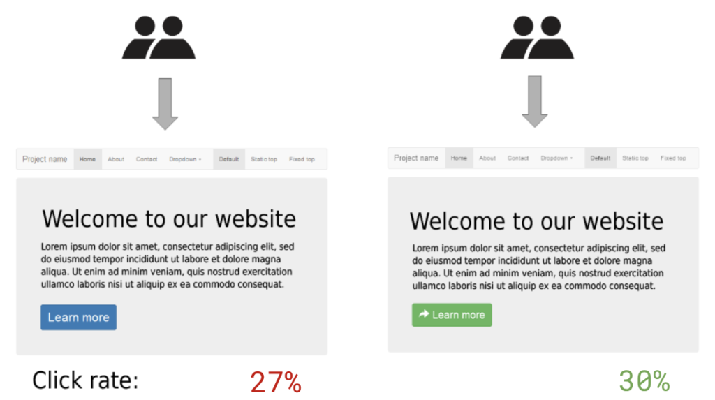
Just looking at those raw percentages, green seems like the clear winner, right?
But hold up! What if those results were just due to chance?
What if, during the week of the test, there was simply a concentration of people who loved the colour green? Maybe next week — a completely random occurrence — prefer blue.
“But…but the numbers…they looked so obvious!” I hear you protesting.
Here’s the deal: we only tested 2,000 people. To be 100% sure the green CTA is better, we’d have to somehow test every potential website visitor on the entire planet.
Since that’s impossible, we have to rely on limited and finite samples and be able to predict how the rest might behave based on what we see in this smaller group.
The Power of Confidence Intervals #
Quantify uncertainty rather than succumbing to it.
Returning to our example, after testing the behaviour of 2,000 people, 27% chose the blue CTA, and 30% chose the green CTA.
At this point, how confident can I be that, over the following months and thousands of users later, the colour green will continue to remain the winning choice?
That’s where the statistical confidence intervals come in.
Confidence intervals help us quantify the uncertainty inherent in testing. They provide a range within which the percentage of people who prefer a certain option (like the green button) is likely to fall.
Let’s proceed with some practical calculations using a statistical calculator.
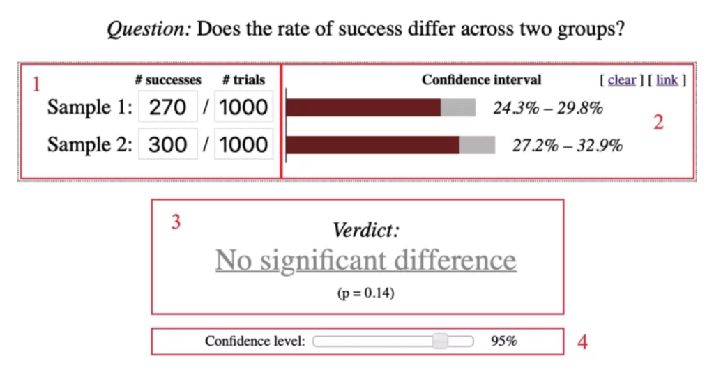
Using Evan Miller’s online calculator, we find that the 95% confidence level gives a confidence interval for the blue button of 24.3% to 29.8%, and for the green, it’s 27.2% to 32.9%.
Those confidence intervals tell you that if we repeated this test 100 times, 95 of those times:
- The blue button’s performance likely falls between 24.3% and 29.8%
- The green button’s performance likely falls between 27.2% and 32.9%
Notice how those ranges overlap?!
We calculated the confidence intervals for each button colour individually. Now, to truly understand if the green button’s performance is a real improvement, not just random luck, we need to compare the confidence intervals of both samples.
Think of it like this: We calculated how confident we are about the range of likely performance for each button. Now, we want to see if those ranges overlap or not. If they do, the difference between the buttons might not be meaningful. If they don’t, it suggests a real difference.
Our test, as shown above, gives us a verdict of “no significant difference” that actually means the test results are NOT statistically significant yet. The difference in clicks could just be random chance!
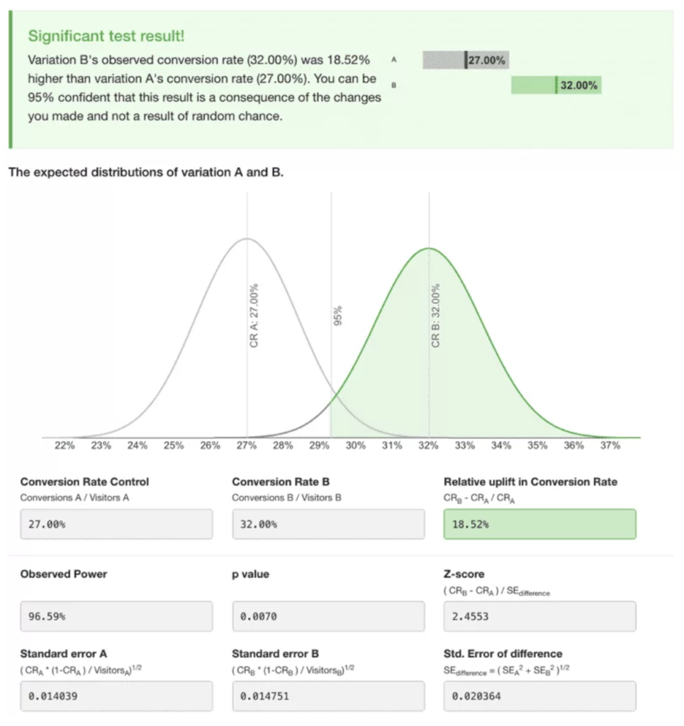
By using a slightly more advanced online calculator, we can see a relative uplift in conversion rate of only 11.11%.

So what do you do? You’ve got two options:
- Abandon the test and make a decision based on gut feeling (not recommended for data-driven marketing).
- Continue the test, gathering more data until we can declare a statistically significant winner. You stop when you have enough traffic/conversions for valid results.
Let’s assume, for example, instead of 300 people clicking the green button, it was 320 out of those 1,000 visitors. Plug those new numbers into the calculator and suddenly boom – the confidence intervals don’t overlap anymore.
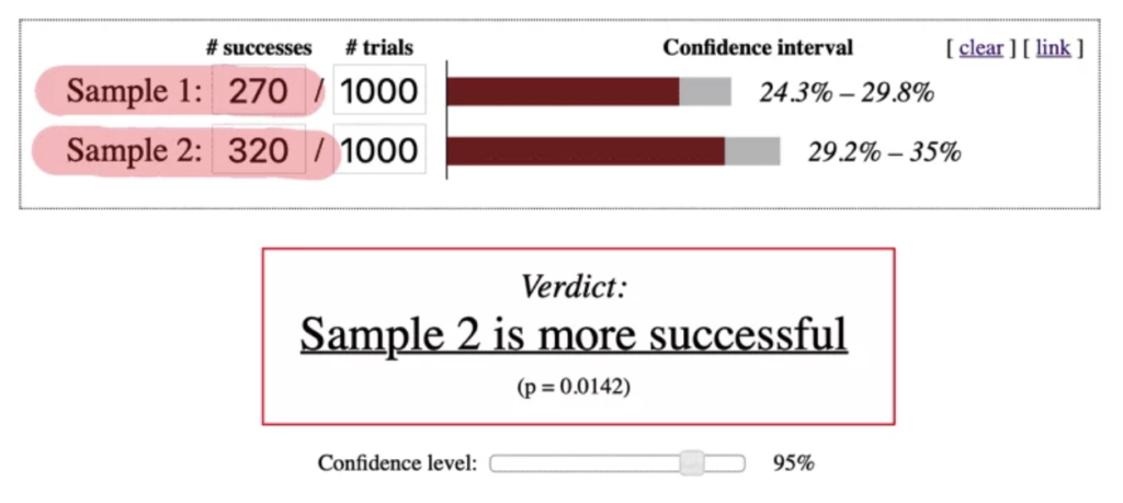
The verdict is “Sample 2 is more successful”. Simplifying everything, it means that the difference in results between the blue (27%) and green (32%) samples is large enough to confidently say people seem to prefer the green button on average.
The Meaning of Confidence Levels #
By using confidence intervals, we shifted from uncertainty to calculated risk.
At this point, we can reasonably assume that if we somehow extended this test to the entire population of potential website visitors, green would remain the winner.
So, you’re telling me that if I now switch to the green button, I can be 100% certain that’s the right call?
Unfortunately not.
Achieving 100% certainty is impossible unless we test the entire population — or the entire applicable user base — there will always be a margin for error.
We choose to have a 95% confidence level which means that the observed change has a 95% chance of being real and only a 5% chance of being purely random.
You may have noticed (I even put it in bold letters) that the confidence level is chosen, not calculated. Typically, the most commonly used confidence level for practical reasons are 90%, 95%, and 99%.
But why is 95% usually used? Isn’t it better to use 99%?
This is a very fair observation. Although a 4% difference seems small, when applied in the real world, it can significantly change the results of a test. It would mean that there is only a 1% chance of making a mistake in the prediction.
However, the problem with conducting tests with a 99% confidence level instead of 95% is that they are much more expensive in terms of resources and time. That’s why, in fields like marketing, design, and UI, a 95% confidence level is considered the industry standard and widely accepted to determine the success or failure of a test.
In sectors like pharmaceuticals, where a person’s health or life is at risk, all tests are conducted with a 99% confidence level to minimise errors.
The Level of Significance #
In the context of A/B testing, the p-value is the metric used to determine the success or failure of an experiment.
Let’s quickly see the process of comparing A/B test results.
There are three steps to take:
- Formulate Two Hypotheses — one ” null” and the other “alternative”;
- Null Hypothesis: CR(B)−CR(A)=0. What this means is: if we subtract the value of A from the value of B, the final result will be zero; ergo, there will be no difference. So, if you observe a difference, it is likely due to chance.
- Alternative Hypothesis: CR(B)>CR(A). It will represent the case in which the value of sample B is higher than sample A.
- Calculate the Probability that the null hypothesis is true — expressed as the “p-value”;
- Compare the p-value with the confidence level expressed as “1−α” — where α (alpha) corresponds to the confidence level.
- If the p-value < 1−α, we consider the test result positive.
Looking at the results from our calculator we can see that:
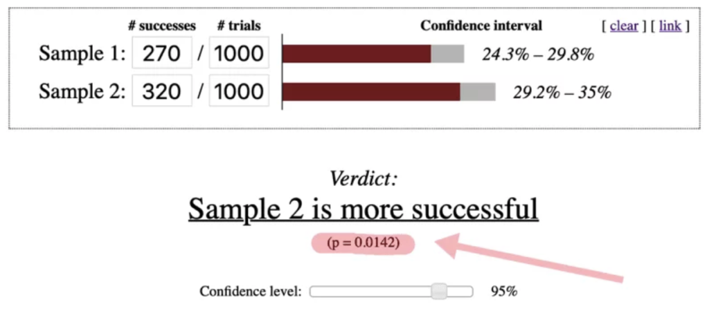
- P-value is 0.0142
- Using a 95% confidence level, 1−α = 0.05 (1 – 0.95 = 0.05).
- 0.0142 < 0.05
What does this mean?
Since the p-value is less than 0.05 (for a 95% confidence level), we can conclude that the outcome of our test is positive and accept that the observed difference is likely due to our changes rather than pure chance.
🤔 In case you were wondering why…
The p-value reported by the second calculator is half that of the first (0.0070 and 0.0142).

The reason is quite simple: in one case, the p-value was calculated using a two-sided test, while in the other, a one-sided test was used.
-
One-sided test: Only looks at a positive difference;

-
Two-sided test: Look at both negative and positive differences.

To illustrate what is meant by uni-sided and bi-sided testing, imagine flipping a coin. If you’re only interested in the probability of getting heads, you’d use a one-sided test. However, if you want to compare how often it comes up heads versus tails, you’d use a two-sided test.
It’s crucial to note that the p-value for a two-sided test will always be double that of a one-sided test. This explains why you might see different p-values (like 0.0070 and 0.0142) from different calculators for the same data – they’re using different types of tests.
The Pitfall of Premature Conclusions #
Did you stop the test as soon as it reached statistical significance?
I hope not… Statistical significance should not dictate when you stop a test.
One common mistake in A/B testing is declaring a winner too soon.
To illustrate this point, consider two approaches to testing website variations:
- Analyse results at 500 visitors and stop if there’s a winner.
- Reaching 1000 before declaring a winner.
This setup leads to four possible scenarios:
Scenario 1 |
Scenario 2 |
Scenario 3 |
Scenario 4 |
|
|---|---|---|---|---|
| After 500 observations | ❌ Insignificant |
❌ Insignificant! |
✅ Significant! |
✅ Significant! |
| After 1000 observations | ❌ Insignificant |
✅ Significant! |
❌ Insignificant |
✅ Significant! |
| End of experiment | ❌ Insignificant |
✅ Significant! |
❌ Insignificant |
✅ Significant! |
- No significant difference at either 500 or 1000 visitors.
- No difference at 500, but significance emerges at 1000.
- Significance at 500, but it disappears by 1000.
- Significance at both 500 and 1000 visitors.
The third scenario highlights the danger of stopping tests prematurely. At 500 observations you are tempted to call the test and crown the winner, but this decision leads to false conclusions. What appears significant at 500 observations may prove to be a random fluctuation when the test runs longer.
This is why declaring the winner too early often risks creating a false illusion about the real outcome of a test.
But how do I know when it’s too early?
The key is to run the test until you reach your full predetermined sample size, not just until you achieve statistical significance.
Pre-determining the Sample Size #
Calculate your sample size upfront.
So, how do you know when you have enough data?
Online calculators can help with this task. The main metrics to consider include:
- Baseline conversion rate: Your current conversion rate.
- Minimum detectable effect (MDE): The minimum improvement you’re aiming for.
Let’s say your current conversion rate is 4%, and you’re aiming for a 5% rate (so 1% improvement) with a 95% confidence level, you’d need to test about 6,328 users per variant. With two variants (A and B), that’s a total of 12,800 users.
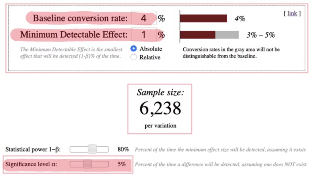
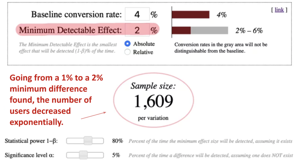
If you don’t have enough traffic to reach these large sample sizes, don’t despair. You can still conduct meaningful tests by aiming for more radical changes between variants. Instead of trying to improve from 4% to 5%, aim for 6%. This larger difference reduces the required sample size significantly – from 12,800 to just 3,200 users.
The takeaway?
Smaller sites should focus on:
-
Testing bold changes that can potentially yield larger improvements.
If you expect a small difference between the two versions, you’ll need a larger sample size compared to expecting a larger difference.

-
Stick to Testing Only Two Variants at a Time
The reason is very simple: The more variations you test against each other, the more traffic you will need.
But not only.
From a mathematical point of view, every time we add a variable, the probability that the outcome of one of them is totally random increases.
For example, conducting a test with a confidence level of 0.05 — 5% — and with 20 variables, the result of one of them would be completely random.
0.05 * 20 = 1.
Simply put: when testing multiple variants simultaneously, the risk of false positives increases. This is known as the Multiple Comparison Problem.

Among the examples that are consistently reported when talking about how a test with too many variations can be misleading, we find the one conducted by Google in 2009 , nicknamed “50 Shades of Blue”.
Since engineers and designers within Google had started having a debate about what shades of blue they should use within paid AdWords advertising links in order to increase clicks, they decided to test all shades of blue.
Considering that they tested 41 shades of blue, the chances that the result found could be considered a false positive corresponded, if applied to a 5% confidence level, to 88%! Which translated means: there is an 88% chance that the observed result is incorrect and not statistically significant.
So, did Google make a mistake?
Actually, no.
The reason why?
With hundreds of millions of users to test, they were eventually able to find an answer that was statistically significant. But if they didn’t have that amount of users to test, they would never have been able to find an answer.
The following image shows the probability of finding a false positive based on the number of variables tested:
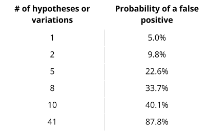
In order to obtain a statistically significant result, we need to change our approach and apply the Bonferroni correction.

As you can see, if we decided to test 41 variables and find a result applying a 5% confidence level using the Bonferroni correction, it would be necessary to apply a 99.9% confidence level.
However, conducting tests of this type requires a huge amount of resources; so much so that, in almost all cases, our tests are impracticable and potentially misleading.
For this reason — and also because it would become extremely complex on a technical and operational level — that it is always advisable to stick to A/B split tests with only two variants.
Pre-determining the Test Duration #
How long should I let my test run?
Once we have identified the number of users needed to test, we will simply have to compare them with the volume of visitors we manage to send to our test pages to understand how many days, approximately, we will have to wait before being able to accept the test results.
Assuming that on average we send about 1,000 visitors per day to both pages (500 to group A and 500 to group B), this means that to reach 12,800 tested individuals, we will need about 13 days.
However, this initial calculation is often not sufficient. You need to keep the following in mind when you calculate how long your experiment should run:
-
Run your test for at least 2 business cycles (usually 2-4 weeks) and for the whole cycle (start and end on the same day)
- You need 12,800 users for your test
- Your site receives 15,000 visits per day
-
Capture Weekly Variations: User behaviour often differs between weekdays and weekends. A full business cycle (typically a week for e-commerce) captures these variations.
-
Account for Different User Types: Different types of users may visit your site at different times of the week. A full cycle ensures you’re considering all user behaviours.
-
Mitigate Unusual Events: Longer test durations help smooth out the effects of any unusual events or short-term fluctuations.
-
The Upper Limit on Test Duration
While it’s important not to end tests too early, running them for too long can also be problematic:
-
Cookie Deletion: Tests running longer than 3-4 weeks risk sample pollution due to cookie deletion.
I only say you need 1,000 conversions per month at least because if you have less, you have to test for 6-7 weeks just to get enough traffic. In that time, people delete cookies. So, you already have sample pollution. Within 2 weeks, you can get a 10% dropout of people deleting cookies and that can really affect your sample quality as well.

-
Changing Conditions: The longer a test runs, the more likely external factors could influence results.
Look at the graph, look for consistency of data, and look for lack of inflection points (comparative analysis). Make sure you have at least 1 week of consistent data (that is not the same as just one week of data).
You cannot replace understanding patterns, looking at the data, and understanding its meaning. Nothing can replace the value of just eyeballing your data to make sure you are not getting spiked on a single day and that your data is consistent. This human level check gives you the context that helps correct against so many imperfections that just looking at the end numbers leaves you open for.
-
Let’s consider a high-traffic scenario:
In this scenario, technically, you could reach your required sample size in less than 24 hours.
However, stopping the test this quickly would be a mistake. Here’s why:
Tests run best in full-week increments since day-of-week and day-of-month present seasonality factors. I perform discovery to better understand the buying cycle duration and target audience daily context (e.g. work schedules, school activities, child/adult bedtimes, biweekly/bimonthly paychecks, etc.) before setting test dates and times.

Therefore, determining the right test duration is a balancing act. You need to run the test long enough to gather sufficient data and account for cyclical variations in user behaviour, but not so long that you risk sample pollution.
As a general rule, aim to complete your test within 2-4 weeks to balance the need for comprehensive data with the risk of sample pollution.
Conclusion #
A/B testing is a powerful tool used to reduce the uncertainty in decision making.
However, as explored, effective testing requires careful planning, patience, and a nuanced understanding of statistical principles.
It’s crucial to remember that data, while invaluable, is not infallible.
As Nassim Taleb wisely noted, “… , when you think you know more than you do, you are fragile (to error).”
